Detection
•Functions and parameters contained in
this package:
In[1]:=
![PackageFunctions[Detection, 2]](HTMLFiles/index_1.gif)
Out[1]//DisplayForm=
![[Graphics:HTMLFiles/index_2.gif]](HTMLFiles/index_2.gif)
•Package functions and their basic documentation
along with simple examples
•BinaryDetectorOptimalM
In[2]:=

![BinaryDetectorOptimalM[DetectionModel, n, Pfa]](HTMLFiles/index_4.gif)
![[Graphics:HTMLFiles/index_5.gif]](HTMLFiles/index_5.gif)
In[3]:=
![BinaryDetectorOptimalM[Swerling0, 20, 1/10^5]](HTMLFiles/index_6.gif)
Out[3]=

In[4]:=
![BinaryDetectorOptimalM[Swerling2, 20, 1/10^5]](HTMLFiles/index_8.gif)
Out[4]=

•BinaryDetectorProbabilityFunction
![[Graphics:HTMLFiles/index_10.gif]](HTMLFiles/index_10.gif)
In[5]:=
![BinaryDetectorProbabilityFunction[n, m, p]](HTMLFiles/index_11.gif)
Out[5]=
![(1 - p)^(-m + n) p^m Binomial[n, m] Gamma[1 + m] Hypergeometric2F1Regularized[1, m - n, 1 + m, p/(-1 + p)]](HTMLFiles/index_12.gif)
•BinaryDetectorSinglePulsePfa
![[Graphics:HTMLFiles/index_13.gif]](HTMLFiles/index_13.gif)
In[6]:=
![BinaryDetectorSinglePulsePfa[5, 2, 10^-6]](HTMLFiles/index_14.gif)
Out[6]=

•BinaryDetector
![[Graphics:HTMLFiles/index_16.gif]](HTMLFiles/index_16.gif)
In[7]:=
![DetectionProbability[{BinaryDetector[SwerlingModel2, 4], 5}, {3, 1/100000}]](HTMLFiles/index_17.gif)
Out[7]=

•CentralMomentsToLaplaceCharacteristicFunction
![[Graphics:HTMLFiles/index_19.gif]](HTMLFiles/index_19.gif)
In[8]:=
![CentralMomentsToLaplaceCharacteristicFunction[{σ^2, κ}, μ, λ]](HTMLFiles/index_20.gif)
Out[8]=
•Central
![[Graphics:HTMLFiles/index_22.gif]](HTMLFiles/index_22.gif)
In[9]:=
![PackagesAndFunctionsWithOption[MomentMethod]](HTMLFiles/index_23.gif)
Out[9]//DisplayForm=
![[Graphics:HTMLFiles/index_24.gif]](HTMLFiles/index_24.gif)
•CentralToNonCentral
![[Graphics:HTMLFiles/index_25.gif]](HTMLFiles/index_25.gif)
In[10]:=
![CentralToNonCentral[2]](HTMLFiles/index_26.gif)
Out[10]=
![-MomentNonCentral[1]^2 + MomentNonCentral[2]](HTMLFiles/index_27.gif)
In[11]:=
![CentralToNonCentral[2, m]](HTMLFiles/index_28.gif)
Out[11]=
![-m[1]^2 + m[2]](HTMLFiles/index_29.gif)
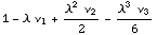
This can be expressed in a more conventional form
by writing μ for the mean and σ for the standard deviation. We
then use an abbreviated notation for higher order central moments:

In[12]:=
![Clear[σ, μ] ; m[1] := μ ; m[2] := σ^2 ; m[i_] := ν _ i ; CentralToNonCentral[2, m]](HTMLFiles/index_31.gif)
Out[16]=

In[17]:=
![CentralToNonCentral[3, m]](HTMLFiles/index_33.gif)
Out[17]=

Arbitraty higher order expressions can easilly be
generated:
In[18]:=
![CentralToNonCentral[15, m]](HTMLFiles/index_35.gif)
Out[18]=

One practical purpose of this function is to transform
data taken for the moments of a distribution from one form to another. For
example the data may be from explicit measurements of the pulse-to-pulse
fluctuations of the radar cross section of a realistic target. These
data can then be used to construct the LaplaceCharacteristicFunction
for this target (using CentralMomentsToLaplaceCharacteristicFunction)
which is then used in the EdgeworthDetectionExpansion or the EdgeworthProbabilityExpansion
to construct a detection model for this target (using MakeEdgeworthDetectionExpansion
or MakeEdgeworthDetectionExpansionCode).
•ChiSquareModel
![[Graphics:HTMLFiles/index_37.gif]](HTMLFiles/index_37.gif)
•CoherentDetector
![[Graphics:HTMLFiles/index_38.gif]](HTMLFiles/index_38.gif)
•CoherentDetectorFunction
![[Graphics:HTMLFiles/index_39.gif]](HTMLFiles/index_39.gif)
Usage message for CoherentDetectorFunction
•CorrelationMatrix
![[Graphics:HTMLFiles/index_40.gif]](HTMLFiles/index_40.gif)
In[19]:=
![CorrelationMatrix[CorrelationFunction, 2]](HTMLFiles/index_41.gif)
Out[19]=
![CorrelationMatrix[CorrelationFunction, 2]](HTMLFiles/index_42.gif)
In[20]:=
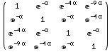
![CorrelationMatrix[χ[#1, #2] &, 3] // MatrixForm](HTMLFiles/index_43.gif)
Out[20]//MatrixForm=
![( χ[1, 1] χ[1, 2] χ[1, 3] ) χ[2, 1] χ[2, 2] χ[2, 3] χ[3, 1] χ[3, 2] χ[3, 3]](HTMLFiles/index_44.gif)
•Cumulant
![[Graphics:HTMLFiles/index_45.gif]](HTMLFiles/index_45.gif)
In[21]:=
![Cumulant[9, m]](HTMLFiles/index_46.gif)
Out[21]=
•DetectionModels
![[Graphics:HTMLFiles/index_48.gif]](HTMLFiles/index_48.gif)
In[22]:=
![DetectionModels[]](HTMLFiles/index_49.gif)
Out[22]=

•DetectionProbabilityCalculator
![[Graphics:HTMLFiles/index_51.gif]](HTMLFiles/index_51.gif)
In[16]:=
![DetectionProbabilityCalculator[]](HTMLFiles/index_52.gif)
Out[16]=
![NotebookObject[<< Detection Probability Calculator >>]](HTMLFiles/index_53.gif)
![[Graphics:HTMLFiles/index_54.gif]](HTMLFiles/index_54.gif)
•DetectionProbabilityReport
![[Graphics:HTMLFiles/index_55.gif]](HTMLFiles/index_55.gif)
In[24]:=
![DetectionProbabilityReport[{5}, {5.0, 10^(-3)}]](HTMLFiles/index_56.gif)
![[Graphics:HTMLFiles/index_57.gif]](HTMLFiles/index_57.gif)
•DetectionProbability
![[Graphics:HTMLFiles/index_58.gif]](HTMLFiles/index_58.gif)
Coherent Detector
In[25]:=
![DetectionProbability[{CoherentDetector, 1}, {snr, pfa}]](HTMLFiles/index_59.gif)
Out[25]=
![DetectionProbability[{CoherentDetector, 1}, {snr, pfa}]](HTMLFiles/index_60.gif)
In[26]:=
![DetectionProbability[{CoherentDetector, 2}, {snr, pfa}]](HTMLFiles/index_61.gif)
Out[26]=
![DetectionProbability[{CoherentDetector, 2}, {snr, pfa}]](HTMLFiles/index_62.gif)
In[27]:=
![DetectionProbability[{CoherentDetector, 3}, {snr, pfa}]](HTMLFiles/index_63.gif)
Out[27]=
![DetectionProbability[{CoherentDetector, 3}, {snr, pfa}]](HTMLFiles/index_64.gif)
Swerling 0
In[28]:=
![DetectionProbability[{SwerlingModel0, 1}, {snr, pfa}]](HTMLFiles/index_65.gif)
Out[28]=
![MarcumQProbabilityFunction[1, snr, -Log[pfa], {ComputationMethod -> Automatic}]](HTMLFiles/index_66.gif)
In[29]:=
![DetectionProbability[{SwerlingModel0, 2}, {snr, pfa}]](HTMLFiles/index_67.gif)
Out[29]=
![MarcumQProbabilityFunction[2, snr, -1 - ProductLog[-1, -pfa/e], {ComputationMethod -> Automatic}]](HTMLFiles/index_68.gif)
In[30]:=
![DetectionProbability[{SwerlingModel0, 3}, {snr, pfa}]](HTMLFiles/index_69.gif)
Out[30]=
![MarcumQProbabilityFunction[3, snr, DetectionThreshold[{SquareLawDetector, 3}, pfa], {ComputationMethod -> Automatic}]](HTMLFiles/index_70.gif)
Swerling 1
In[31]:=
![DetectionProbability[{SwerlingModel1, 1}, {snr, pfa}]](HTMLFiles/index_71.gif)
Out[31]=

In[32]:=
![DetectionProbability[{SwerlingModel1, 2}, {snr, pfa}]](HTMLFiles/index_73.gif)
Out[32]=
![(e^(1 + ProductLog[-1, -pfa/e]) (-1 + e^(2 snr (-1 - ProductLog[-1, -pfa/e]))/(1 + 2 snr) (1 + 2 snr)))/(2 snr)](HTMLFiles/index_74.gif)
In[33]:=
![DetectionProbability[{SwerlingModel1, 3}, {snr, pfa}]](HTMLFiles/index_75.gif)
Out[33]=
![GammaRegularized[2, DetectionThreshold[{SquareLawDetector, 3}, pfa]] + e^(-DetectionThreshold[ ... snr))^2 (1 - GammaRegularized[2, DetectionThreshold[{SquareLawDetector, 3}, pfa]/(1 + 1/(3 snr))])](HTMLFiles/index_76.gif)
Swerling 2
In[34]:=
![DetectionProbability[{SwerlingModel2, 1}, {snr, pfa}]](HTMLFiles/index_77.gif)
Out[34]=

In[35]:=
![DetectionProbability[{SwerlingModel2, 2}, {snr, pfa}]](HTMLFiles/index_79.gif)
Out[35]=
![GammaRegularized[2, (-1 - ProductLog[-1, -pfa/e])/(1 + snr)]](HTMLFiles/index_80.gif)
In[36]:=
![DetectionProbability[{SwerlingModel2, 3}, {snr, pfa}]](HTMLFiles/index_81.gif)
Out[36]=
![GammaRegularized[3, DetectionThreshold[{SquareLawDetector, 3}, pfa]/(1 + snr)]](HTMLFiles/index_82.gif)
Swerling 3
In[37]:=
![DetectionProbability[{SwerlingModel3, 1}, {snr, pfa}]](HTMLFiles/index_83.gif)
Out[37]=
![pfa^1/(1 + snr/2) (1 - (2 snr Log[pfa])/(2 + snr)^2)](HTMLFiles/index_84.gif)
In[38]:=
![DetectionProbability[{SwerlingModel3, 2}, {snr, pfa}]](HTMLFiles/index_85.gif)
Out[38]=
![e^(-(-1 - ProductLog[-1, -pfa/e])/(1 + snr)) (1 + (-1 - ProductLog[-1, -pfa/e])/(1 + snr))](HTMLFiles/index_86.gif)
In[39]:=
![DetectionProbability[{SwerlingModel3, 3}, {snr, pfa}]](HTMLFiles/index_87.gif)
Out[39]=
![e^(-DetectionThreshold[{SquareLawDetector, 3}, pfa]/(1 + (3 snr)/2)) (1 + 2/(3 snr)) (1 - 2/(3 snr) + DetectionThreshold[{SquareLawDetector, 3}, pfa]/(1 + (3 snr)/2))](HTMLFiles/index_88.gif)
Swerling 4
In[40]:=
![DetectionProbability[{SwerlingModel4, 1}, {snr, pfa}]](HTMLFiles/index_89.gif)
Out[40]=
![pfa^1/(1 + snr/2) (1 - (2 snr Log[pfa])/(2 + snr)^2)](HTMLFiles/index_90.gif)
In[41]:=
![DetectionProbability[{SwerlingModel4, 2}, {snr, pfa}]](HTMLFiles/index_91.gif)
Out[41]=
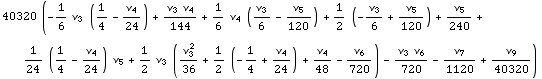
![1 - 1/(1 + snr/2)^2 (2 (1/2 (1 - GammaRegularized[2, (-1 - ProductLog[-1, -pfa/e])/(1 + snr/2) ... )/(1 + snr/2)]) + 1/8 snr^2 (1 - GammaRegularized[4, (-1 - ProductLog[-1, -pfa/e])/(1 + snr/2)])))](HTMLFiles/index_92.gif)
In[42]:=
![DetectionProbability[{SwerlingModel4, 3}, {snr, pfa}]](HTMLFiles/index_93.gif)
Out[42]=
![1 - 1/(1 + snr/2)^3 (6 (1/6 (1 - GammaRegularized[3, DetectionThreshold[{SquareLawDetector, 3} ... /48 snr^3 (1 - GammaRegularized[6, DetectionThreshold[{SquareLawDetector, 3}, pfa]/(1 + snr/2)])))](HTMLFiles/index_94.gif)
 versus snr at a value of
  for a single pulse:
In[43]:=
![WeibullPlot[Evaluate[DetectionProbability[{SwerlingModel4, 1}, {snr, 10^(-5)}]], {snr, 1, 20}, Frame -> True, Axes -> False, FrameLabel -> {SNR, Pd}, AspectRatio -> GoldenRatio] ;](HTMLFiles/index_97.gif)
![[Graphics:HTMLFiles/index_98.gif]](HTMLFiles/index_98.gif)
 versus snr at a value of
  for a 10 pulses:
In[44]:=
![WeibullPlot[Evaluate[DetectionProbability[{SwerlingModel4, 10}, {snr, 10^(-5)}]], {snr, 1, 20}, Frame -> True, Axes -> False, FrameLabel -> {SNR, Pd}, AspectRatio -> GoldenRatio] ;](HTMLFiles/index_101.gif)
![[Graphics:HTMLFiles/index_102.gif]](HTMLFiles/index_102.gif)
•Detection
![[Graphics:HTMLFiles/index_103.gif]](HTMLFiles/index_103.gif)
•DetectionThreshold
![[Graphics:HTMLFiles/index_104.gif]](HTMLFiles/index_104.gif)
In[45]:=
![DetectionThreshold[{SquareLawDetector, 4}, 10^(-3)]](HTMLFiles/index_105.gif)
Out[45]=

In[46]:=
![DetectionThreshold[{CoherentDetector, 4}, 10^(-3)] // N](HTMLFiles/index_107.gif)
Out[46]=

In[47]:=
![DetectionThreshold[{BinaryDetector[4], 4}, 10^(-3)]](HTMLFiles/index_109.gif)
Out[47]=
![(3 Log[10])/4](HTMLFiles/index_110.gif)
•Detectors
![[Graphics:HTMLFiles/index_111.gif]](HTMLFiles/index_111.gif)
In[48]:=
![Detectors[]](HTMLFiles/index_112.gif)
Out[48]=

•EdgeworthCumulativeExpansion
![[Graphics:HTMLFiles/index_114.gif]](HTMLFiles/index_114.gif)
In[49]:=
![EdgeworthCumulativeExpansion[2, t]](HTMLFiles/index_115.gif)
Out[49]=
![1/2 (1 + Erf[t/2^(1/2)])](HTMLFiles/index_116.gif)
In[50]:=
![EdgeworthCumulativeExpansion[3, t]](HTMLFiles/index_117.gif)
Out[50]=
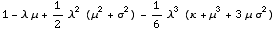
![1/2 (1 + Erf[t/2^(1/2)]) - (e^(-t^2/2) (-2 + 2 t^2) MomentCentral[3])/(12 (2 π)^(1/2))](HTMLFiles/index_118.gif)
In[51]:=
![EdgeworthCumulativeExpansion[4, t]](HTMLFiles/index_119.gif)
Out[51]=
![(e^(-t^2/2) (-6 2^(1/2) t + 2 2^(1/2) t^3))/(32 π^(1/2)) + 1/2 (1 + Erf[t/2^(1/2)]) - (e^ ... 576 π^(1/2)) - (e^(-t^2/2) (-6 2^(1/2) t + 2 2^(1/2) t^3) MomentCentral[4])/(96 π^(1/2))](HTMLFiles/index_120.gif)
•EdgeworthDetectionExpansion
![[Graphics:HTMLFiles/index_121.gif]](HTMLFiles/index_121.gif)
In[52]:=
![EdgeworthDetectionExpansion[1, t]](HTMLFiles/index_122.gif)
Out[52]=
![1 + 1/2 (-1 - Erf[t/2^(1/2)])](HTMLFiles/index_123.gif)
In[53]:=
![EdgeworthDetectionExpansion[2, t]](HTMLFiles/index_124.gif)
Out[53]=
![1 + 1/2 (-1 - Erf[t/2^(1/2)])](HTMLFiles/index_125.gif)
In[54]:=
![EdgeworthDetectionExpansion[3, t]](HTMLFiles/index_126.gif)
Out[54]=
![1 + 1/2 (-1 - Erf[t/2^(1/2)]) + (e^(-t^2/2) (-2 + 2 t^2) MomentCentral[3])/(12 (2 π)^(1/2))](HTMLFiles/index_127.gif)
•EdgeworthProbabilityExpansion
![[Graphics:HTMLFiles/index_128.gif]](HTMLFiles/index_128.gif)
In[55]:=
![EdgeworthDetectionExpansion[1, t]](HTMLFiles/index_129.gif)
Out[55]=
![1 + 1/2 (-1 - Erf[t/2^(1/2)])](HTMLFiles/index_130.gif)
In[56]:=
![EdgeworthDetectionExpansion[2, t]](HTMLFiles/index_131.gif)
Out[56]=
![1 + 1/2 (-1 - Erf[t/2^(1/2)])](HTMLFiles/index_132.gif)
In[57]:=
![EdgeworthDetectionExpansion[3, t]](HTMLFiles/index_133.gif)
Out[57]=
![1 + 1/2 (-1 - Erf[t/2^(1/2)]) + (e^(-t^2/2) (-2 + 2 t^2) MomentCentral[3])/(12 (2 π)^(1/2))](HTMLFiles/index_134.gif)
•EdgeworthTerms
![[Graphics:HTMLFiles/index_135.gif]](HTMLFiles/index_135.gif)
In[58]:=
![EdgeworthTerms[k, Phi, semiInvariant]](HTMLFiles/index_136.gif)
Out[58]=
![EdgeworthTerms[k, Phi, semiInvariant]](HTMLFiles/index_137.gif)
In[59]:=
![EdgeworthTerms[3, Phi, semiInvariant]](HTMLFiles/index_138.gif)
Out[59]=
![Phi[0] - 1/6 Phi[3] semiInvariant[3]](HTMLFiles/index_139.gif)
•ExponentialCorrelationMatrix
![[Graphics:HTMLFiles/index_140.gif]](HTMLFiles/index_140.gif)
In[60]:=
![ExponentialCorrelationMatrix[α, 4] // MatrixForm](HTMLFiles/index_141.gif)
Out[60]//MatrixForm=

•FalseAlarmNumberToFalseAlarmProbability
![[Graphics:HTMLFiles/index_143.gif]](HTMLFiles/index_143.gif)
In[61]:=
![FalseAlarmNumberToFalseAlarmProbability[n _ fa]](HTMLFiles/index_144.gif)
Out[61]=

•FalseAlarmProbability
![[Graphics:HTMLFiles/index_146.gif]](HTMLFiles/index_146.gif)
In[62]:=
![FalseAlarmProbability[{SquareLawDetector, 4}, τ]](HTMLFiles/index_147.gif)
Out[62]=
![GammaRegularized[4, τ]](HTMLFiles/index_148.gif)
In[63]:=
![FalseAlarmProbability[{CoherentDetector, 4}, τ]](HTMLFiles/index_149.gif)
Out[63]=

•FalseAlarmProbabilityToFalseAlarmNumber
![[Graphics:HTMLFiles/index_151.gif]](HTMLFiles/index_151.gif)
In[64]:=
![FalseAlarmProbabilityToFalseAlarmNumber[p _ fa]](HTMLFiles/index_152.gif)
Out[64]=
![-Log[2]/Log[1 - p _ fa]](HTMLFiles/index_153.gif)
•GammaExpansion
![[Graphics:HTMLFiles/index_154.gif]](HTMLFiles/index_154.gif)
In[65]:=
![PackagesAndFunctionsWithOption[ComputationMethod]](HTMLFiles/index_155.gif)
Out[65]//DisplayForm=
![[Graphics:HTMLFiles/index_156.gif]](HTMLFiles/index_156.gif)
•GaussianCorrelationMatrix
![[Graphics:HTMLFiles/index_157.gif]](HTMLFiles/index_157.gif)
In[66]:=
![GaussianCorrelationMatrix[α, 4] // MatrixForm](HTMLFiles/index_158.gif)
Out[66]//MatrixForm=
•GCFunction
![[Graphics:HTMLFiles/index_160.gif]](HTMLFiles/index_160.gif)
In[67]:=
![PackagesAndFunctionsWithOption[GCFunction]](HTMLFiles/index_161.gif)
Out[67]//DisplayForm=
![[Graphics:HTMLFiles/index_162.gif]](HTMLFiles/index_162.gif)
•GramCharlierCumulativeExpansion
![[Graphics:HTMLFiles/index_163.gif]](HTMLFiles/index_163.gif)
In[68]:=
![GramCharlierCumulativeExpansion[1, t]](HTMLFiles/index_164.gif)
Out[68]=
![1/2 (1 + Erf[t/2^(1/2)])](HTMLFiles/index_165.gif)
In[69]:=
![GramCharlierCumulativeExpansion[2, t]](HTMLFiles/index_166.gif)
Out[69]=
![1/2 (1 + Erf[t/2^(1/2)])](HTMLFiles/index_167.gif)
In[70]:=
![GramCharlierCumulativeExpansion[3, t]](HTMLFiles/index_168.gif)
Out[70]=
![1/2 (1 + Erf[t/2^(1/2)]) - (e^(-t^2/2) (-1 + t^2) MomentCentral[3])/(6 (2 π)^(1/2))](HTMLFiles/index_169.gif)
•GramCharlierDetectionExpansion
![[Graphics:HTMLFiles/index_170.gif]](HTMLFiles/index_170.gif)
In[71]:=
![GramCharlierDetectionExpansion[1, t]](HTMLFiles/index_171.gif)
Out[71]=
![1 + 1/2 (-1 - Erf[t/2^(1/2)])](HTMLFiles/index_172.gif)
In[72]:=
![GramCharlierDetectionExpansion[2, t]](HTMLFiles/index_173.gif)
Out[72]=
![1 + 1/2 (-1 - Erf[t/2^(1/2)])](HTMLFiles/index_174.gif)
In[73]:=
![GramCharlierDetectionExpansion[3, t]](HTMLFiles/index_175.gif)
Out[73]=
![1 + 1/2 (-1 - Erf[t/2^(1/2)]) + (e^(-t^2/2) (-1 + t^2) MomentCentral[3])/(6 (2 π)^(1/2))](HTMLFiles/index_176.gif)
•GramCharlierFunction
![[Graphics:HTMLFiles/index_177.gif]](HTMLFiles/index_177.gif)
In[74]:=
![GramCharlierFunction[1, t]](HTMLFiles/index_178.gif)
Out[74]=

In[75]:=
![GramCharlierFunction[2, t]](HTMLFiles/index_180.gif)
Out[75]=

In[76]:=
![GramCharlierFunction[3, t]](HTMLFiles/index_182.gif)
Out[76]=
•GramCharlierProbabilityExpansion
![[Graphics:HTMLFiles/index_184.gif]](HTMLFiles/index_184.gif)
In[77]:=
![GramCharlierProbabilityExpansion[1, t]](HTMLFiles/index_185.gif)
Out[77]=

In[78]:=
![GramCharlierProbabilityExpansion[2, t]](HTMLFiles/index_187.gif)
Out[78]=

In[79]:=
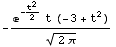
![GramCharlierProbabilityExpansion[3, t]](HTMLFiles/index_189.gif)
Out[79]=
![e^(-t^2/2)/(2 π)^(1/2) + (e^(-t^2/2) t (-3 + t^2) MomentCentral[3])/(6 (2 π)^(1/2))](HTMLFiles/index_190.gif)
•LaplaceCharacteristicFunction
![[Graphics:HTMLFiles/index_191.gif]](HTMLFiles/index_191.gif)
In[80]:=
![LaplaceCharacteristicFunction[{ModelType, NumberOfPulses}, SignalToNoiseRatio, LaplaceVariable]](HTMLFiles/index_192.gif)
Out[80]=
![LaplaceCharacteristicFunction[{ModelType, NumberOfPulses}, SignalToNoiseRatio, LaplaceVariable]](HTMLFiles/index_193.gif)
In[81]:=
![LaplaceCharacteristicFunction[{MarcumModel, n}, s, λ]](HTMLFiles/index_194.gif)
Out[81]=

•LinearDetectorFunction
![[Graphics:HTMLFiles/index_196.gif]](HTMLFiles/index_196.gif)
Usage message for LinearDetectorFunction
•MakeEdgeworthDetectionExpansionCode
![[Graphics:HTMLFiles/index_197.gif]](HTMLFiles/index_197.gif)
In[82]:=
![MakeEdgeworthDetectionExpansionCode[marcum, {LaplaceCharacteristicFunction[{MarcumModel, n}, s, λ], λ}, τ, 3]](HTMLFiles/index_198.gif)
![[Graphics:HTMLFiles/index_199.gif]](HTMLFiles/index_199.gif)
•MakeEdgeworthDetectionExpansion
![[Graphics:HTMLFiles/index_200.gif]](HTMLFiles/index_200.gif)
In[88]:=
![MakeEdgeworthDetectionExpansion[{LaplaceCharacteristicFunction[{MarcumModel, n}, s, λ], λ}, τ, 1]](HTMLFiles/index_201.gif)
Out[88]=
![1 + 1/2 (-1 - Erf[(-n (1 + s) + τ)/(2^(1/2) (n + 2 n s)^(1/2))])](HTMLFiles/index_202.gif)
In[89]:=
![MakeEdgeworthDetectionExpansion[{LaplaceCharacteristicFunction[{MarcumModel, n}, s, λ], λ}, τ, 3]](HTMLFiles/index_203.gif)
Out[89]=
![1 + (e^(-(-n (1 + s) + τ)^2/(2 (n + 2 n s))) (n + 3 n s) (-2 + (2 (-n (1 + s) + τ)^2 ... 960;)^(1/2) (n + 2 n s)^(3/2)) + 1/2 (-1 - Erf[(-n (1 + s) + τ)/(2^(1/2) (n + 2 n s)^(1/2))])](HTMLFiles/index_204.gif)
•MarcumModel
![[Graphics:HTMLFiles/index_205.gif]](HTMLFiles/index_205.gif)
•Models
![[Graphics:HTMLFiles/index_206.gif]](HTMLFiles/index_206.gif)
In[90]:=
![PackagesAndFunctionsWithOption[Models]](HTMLFiles/index_207.gif)
Out[90]//DisplayForm=
![[Graphics:HTMLFiles/index_208.gif]](HTMLFiles/index_208.gif)
•MomentCentral
![[Graphics:HTMLFiles/index_209.gif]](HTMLFiles/index_209.gif)
•MomentFunction
![[Graphics:HTMLFiles/index_210.gif]](HTMLFiles/index_210.gif)
In[91]:=
![PackagesAndFunctionsWithOption[MomentFunction]](HTMLFiles/index_211.gif)
Out[91]//DisplayForm=
![[Graphics:HTMLFiles/index_212.gif]](HTMLFiles/index_212.gif)
•MomentMethod
![[Graphics:HTMLFiles/index_213.gif]](HTMLFiles/index_213.gif)
The  central moment of a probability distribution of one varialbe
  is
is  where μ is the mean of the distribution.
The  noncentral moment of a probability distribution of one varialbe
 is
is  .
.
In[92]:=
![PackagesAndFunctionsWithOption[MomentMethod]](HTMLFiles/index_220.gif)
Out[92]//DisplayForm=
![[Graphics:HTMLFiles/index_221.gif]](HTMLFiles/index_221.gif)
•MomentNonCentral
![[Graphics:HTMLFiles/index_222.gif]](HTMLFiles/index_222.gif)
•NonCentralMomentsToLaplaceCharacteristicFunction
![[Graphics:HTMLFiles/index_223.gif]](HTMLFiles/index_223.gif)
In[93]:=
![NonCentralMomentsToLaplaceCharacteristicFunction[{ν _ 1, ν _ 2, ν _ 3}, λ]](HTMLFiles/index_224.gif)
Out[93]=
•NonCentral
![[Graphics:HTMLFiles/index_226.gif]](HTMLFiles/index_226.gif)
•NonCentralToCentral
![[Graphics:HTMLFiles/index_227.gif]](HTMLFiles/index_227.gif)
In[94]:=
![NonCentralToCentral[2]](HTMLFiles/index_228.gif)
Out[94]=
![MomentCentral[2] + MomentNonCentral[1]^2](HTMLFiles/index_229.gif)
In[95]:=
![NonCentralToCentral[2, {c, μ}]](HTMLFiles/index_230.gif)
Out[95]=
![c[2] + μ[1]^2](HTMLFiles/index_231.gif)
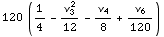
This can be expressed in a more concisely using an
abbreviated notation for higher order central moments:  . .
In[96]:=
![Clear[σ, μ] ; μ[1] := μ ; c[i_] := χ _ i ; NonCentralToCentral[2, {c, μ}]](HTMLFiles/index_233.gif)
Out[99]=

In[100]:=
![NonCentralToCentral[3, {c, μ}]](HTMLFiles/index_235.gif)
Out[100]=

Arbitraty higher order expressions can easilly be
generated:
In[101]:=
![NonCentralToCentral[15, {c, μ}]](HTMLFiles/index_237.gif)
Out[101]=

As with the function CentralToNonCentral, one practical
purpose of this function is to transform data taken for the moments
of a distribution from one form to another. For example
the data may be from explicit measurements of the pulse-to-pulse
fluctuations of the radar cross section of a realistic target. These
data can then be used to construct the LaplaceCharacteristicFunction
for this target (using CentralMomentsToLaplaceCharacteristicFunction)
which is then used in the EdgeworthDetectionExpansion or the EdgeworthProbabilityExpansion
to construct a detection model for this target (using MakeEdgeworthDetectionExpansion
or MakeEdgeworthDetectionExpansionCode).
•NonFluctuatingModel
![[Graphics:HTMLFiles/index_239.gif]](HTMLFiles/index_239.gif)
•PositiveIntegerOrExpressionQ
![[Graphics:HTMLFiles/index_240.gif]](HTMLFiles/index_240.gif)
Usage message for PositiveIntegerOrExpressionQ
•PositiveOrExpressionQ
![[Graphics:HTMLFiles/index_241.gif]](HTMLFiles/index_241.gif)
Usage message for PositiveOrExpressionQ
•ProbabilityOfDetection
![[Graphics:HTMLFiles/index_242.gif]](HTMLFiles/index_242.gif)
Usage message for ProbabilityOfDetection
•ProbabilityOfFalseAlarm
![[Graphics:HTMLFiles/index_243.gif]](HTMLFiles/index_243.gif)
Usage message for ProbabilityOfFalseAlarm
•ProbabilityOrExpressionQ
![[Graphics:HTMLFiles/index_244.gif]](HTMLFiles/index_244.gif)
Usage message for ProbabilityOrExpressionQ
•ProbabilityQ
![[Graphics:HTMLFiles/index_245.gif]](HTMLFiles/index_245.gif)
In[102]:=
![ProbabilityQ[1.1]](HTMLFiles/index_246.gif)
Out[102]=

In[103]:=
![ProbabilityQ[1/π]](HTMLFiles/index_248.gif)
Out[103]=

•ProbabilityQWithMessage
![[Graphics:HTMLFiles/index_250.gif]](HTMLFiles/index_250.gif)
Usage message for ProbabilityQWithMessage
•PureSymbolOrExpressionQ
![[Graphics:HTMLFiles/index_251.gif]](HTMLFiles/index_251.gif)
Usage message for PureSymbolOrExpressionQ
•RiceModel
![[Graphics:HTMLFiles/index_252.gif]](HTMLFiles/index_252.gif)
•SemiInvariant
![[Graphics:HTMLFiles/index_253.gif]](HTMLFiles/index_253.gif)
In[104]:=
![SemiInvariant[6, m]](HTMLFiles/index_254.gif)
Out[104]=
In[105]:=
![Cumulant[6, m]](HTMLFiles/index_256.gif)
Out[105]=

•SignalToNoiseReport
![[Graphics:HTMLFiles/index_258.gif]](HTMLFiles/index_258.gif)
In[106]:=
![SignalToNoiseReport[{5}, {.99, 10^(-5)}]](HTMLFiles/index_259.gif)
![[Graphics:HTMLFiles/index_260.gif]](HTMLFiles/index_260.gif)
In[107]:=
![SignalToNoise[{SwerlingModel1, 2}, {.99, 10^(-5)}] // TodB](HTMLFiles/index_261.gif)
Out[107]=

•SignalToNoise
![[Graphics:HTMLFiles/index_263.gif]](HTMLFiles/index_263.gif)
In[108]:=
![SignalToNoise[{Swerling1, 1}, {pd, 10^(-5)}]](HTMLFiles/index_264.gif)
Out[108]=
![-(Log[100000] + Log[pd])/Log[pd]](HTMLFiles/index_265.gif)
In[109]:=
![SignalToNoise[{Swerling1, 1}, {.75, 10^(-5)}]](HTMLFiles/index_266.gif)
Out[109]=

In[110]:=
![pd = DetectionProbability[{SwerlingModel1, 2}, {10, 10^(-5)}] // N](HTMLFiles/index_268.gif)
Out[110]=

In[111]:=
![SignalToNoise[{Swerling1, 2}, {pd, 10^(-5)}]](HTMLFiles/index_270.gif)
Out[111]=

In[112]:=
![pd = DetectionProbability[{SwerlingModel1, 2}, {10, 10^(-5)}] // N](HTMLFiles/index_272.gif)
Out[112]=

In[113]:=
![Options[SignalToNoise]](HTMLFiles/index_274.gif)
Out[113]=

In[114]:=
![SignalToNoise[{Swerling1, 1}, {9/10, 10^(-5)}]](HTMLFiles/index_276.gif)
Out[114]=
![(-Log[10/9] + Log[100000])/Log[10/9]](HTMLFiles/index_277.gif)
•SquareLawDetectorFunction
![[Graphics:HTMLFiles/index_278.gif]](HTMLFiles/index_278.gif)
In[135]:=
![SquareLawDetectorFunction[{x1, x2}]](HTMLFiles/index_279.gif)
Out[135]=
![Abs[x1]^2 + Abs[x2]^2](HTMLFiles/index_280.gif)
•SquareLawDetector
![[Graphics:HTMLFiles/index_281.gif]](HTMLFiles/index_281.gif)
•SquareLawMixedDetector
![[Graphics:HTMLFiles/index_282.gif]](HTMLFiles/index_282.gif)
•Swerling0
![[Graphics:HTMLFiles/index_283.gif]](HTMLFiles/index_283.gif)
•Swerling1
![[Graphics:HTMLFiles/index_284.gif]](HTMLFiles/index_284.gif)
•Swerling2
![[Graphics:HTMLFiles/index_285.gif]](HTMLFiles/index_285.gif)
•Swerling3
![[Graphics:HTMLFiles/index_286.gif]](HTMLFiles/index_286.gif)
•Swerling4
![[Graphics:HTMLFiles/index_287.gif]](HTMLFiles/index_287.gif)
•Swerling5
![[Graphics:HTMLFiles/index_288.gif]](HTMLFiles/index_288.gif)
•SwerlingCompute
![[Graphics:HTMLFiles/index_289.gif]](HTMLFiles/index_289.gif)
•SwerlingModel0
![[Graphics:HTMLFiles/index_290.gif]](HTMLFiles/index_290.gif)
•SwerlingModel1
![[Graphics:HTMLFiles/index_291.gif]](HTMLFiles/index_291.gif)
•SwerlingModel2
![[Graphics:HTMLFiles/index_292.gif]](HTMLFiles/index_292.gif)
•SwerlingModel3
![[Graphics:HTMLFiles/index_293.gif]](HTMLFiles/index_293.gif)
•SwerlingModel4
![[Graphics:HTMLFiles/index_294.gif]](HTMLFiles/index_294.gif)
•SwerlingModel5
![[Graphics:HTMLFiles/index_295.gif]](HTMLFiles/index_295.gif)
|